Aspheric Lens,Standard Aspheric Lens,Positive Meniscus Lenses,High Precision Aspheric Lens Danyang Horse Optical Co., Ltd , https://www.dyhorseoptical.com
Reference compensation circuit in TL431
**Introduction**
TL431 is a three-terminal, adjustable precision voltage reference integrated circuit developed by Texas Instruments. It is known for its excellent thermal stability and is widely used in the market as a voltage regulator. The output voltage of TL431 can be set to a desired value between 2.5V and 36V using two external resistors. This makes it a flexible and reliable component in various electronic applications. Inside the device, there is a bandgap reference that plays a crucial role in determining the overall performance. The temperature stability and accuracy of the reference directly affect the reliability and efficiency of the entire system, making a high-performance reference essential for optimal operation.
**1. Temperature-Compensated Reference Source**
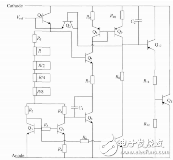
*Figure 1: TL431 schematic*
This circuit employs a highly accurate reference source (as shown in Figure 1). Compared to traditional reference circuits, this design includes nonlinear temperature compensation. The nonlinearity involves both exponential curvature compensation and second-order compensation. Figure 2 illustrates a schematic with curvature compensation.
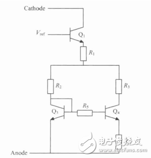
*Figure 2: Curvature compensation reference source*
As shown in Figure 2, resistors R3 and R2 have the same voltage drop, and their resistance ratio is R3:R2 = 3:1. The current through these resistors, I3 and I2, has a ratio of 1:3. The current through resistor R1 is the sum of I3 and I2: I1 = I3 + I2.
The reference voltage expression is given by:
**Vref = Vbe1 + Vbe3 + I1R1 + I2R2 (1)**
Using Kirchhoff’s Voltage Law (KVL), the current through resistor R3 can be calculated. Since Ib = Ic / β, where β is the transistor's current gain:
**I3 = βVT ln M / [R5 + (β + 1)R4] (2)**
Here, M represents the area ratio of the emitter regions of Q3 and Q4. From I3, we can derive I1 and I2. Finally, the reference voltage expression becomes:
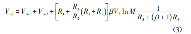
In the above formula, both Vbe and β are temperature-dependent variables, and their expressions are:
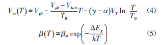
Where α and γ are process-dependent but temperature-independent constants, and Vg0 and Vbe represent the silicon bandgap voltage and base-emitter voltage, respectively. Substituting equations (4) and (5) into equation (1) gives the temperature-dependent expression of the reference voltage:
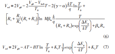
Here, A and B are constant terms, while K1 and K2 can be adjusted through resistor values. As seen in the formula, the reference voltage consists of three components: a constant term, a linear term, and a nonlinear term. These terms are expressed as follows:
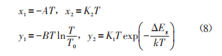
By carefully adjusting these parameters, the temperature drift of the reference voltage can be minimized, ensuring stable and accurate performance over a wide range of operating conditions.