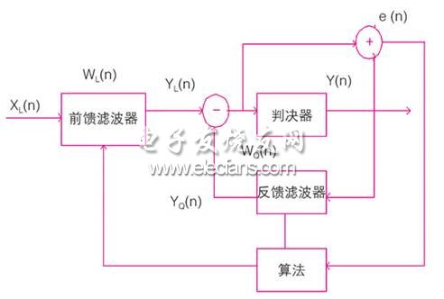
Underwater acoustic channel is a very complex time, space and frequency-variable parameter random multi-channel transmission channel. Adaptive equalization can make full use of limited bandwidth and become a powerful method in underwater acoustic signal processing. Its basic idea is to make the frequency characteristics of the equalizer equal to the reciprocal of the channel frequency characteristics by adjusting the parameters (weights), thereby indirectly obtaining the channel characteristics to eliminate multipath interference [3]. Due to the difference of equalization algorithm and equalization structure, how to improve the algorithm and structure to achieve the best equalization effect has been the focus of equalizer research. In this paper, we compare the advantages and disadvantages of traditional lms decision feedback equalizer and nlms decision feedback equalizer in terms of actual signal processing for the actual data collected by underwater acoustic communication, and adjust the equalizer parameters to achieve the best overall performance. Algorithm principle Principle of adaptive decision feedback equalizer Most literature mentions that in underwater acoustic communication, the equalizer can solve the problem of inter-symbol interference, but the structure of the equalizer and the algorithm of the equalizer have always been problems that people have studied. The principle of the decision feedback equalizer is shown in Figure 1. Figure 1 Principle block diagram of adaptive decision feedback equalizer In the figure, assume that the input signal vector of the filter is xl (n) = [xl (n) xl (n-1) ... xl (1)] t, the expected signal is d (n), and the filter weight vector is wl (n) = [wl0 (n) wl1 (n) ... wl (n-1) (n)] t, then the output yl (n) of the feedforward filter is: yl (n) = xt (n) wl ( n), the error signal after output is: e (n) = d (n) -yl (n). At this time, the output of the equalizer is y (n) = yl (n) -yq (n), where yq (n) is the output of the feedback filter. It can be seen from the figure that in the filtering process, the adaptive filter calculates its response to the input and obtains the estimated error signal by comparing with the expected response; in the adaptive process, the estimated error signal enters the feedback filter again as The input signal of the filter is fed back to obtain a new output, and finally the difference between the output results of the two filters is used as the output of the entire equalizer. Generally, the mean square value of the estimated error j = e [e2 (n)] is used as the performance function of the adaptive filter, and the steepest descent method (w (n + 1) = w (n) -μ (n), μ Is the convergence factor, used to adjust the step size of the adaptive iteration; (n) is the gradient of the performance function) iteratively finds its extreme value; in a geometric sense, the result of iteratively adjusting the weight coefficient vector is to make the system mean square error The gradient decreases in the opposite direction and eventually reaches the minimum mean square error jmin. Traditional lms algorithm and normalized lms algorithm For stationary processes, the least mean square (lms) algorithm [4] [5] is to directly use the e2 (n) obtained from single sampling data instead of the mean square error j (n) to estimate the gradient . The algorithm flow is as follows: (1) According to the known data, the desired signal d (n) and the input signal vector x (n) of the filter = [x (n) x (n-1) ... x (1)] t, set the convergence factor μ ( 0 <μ (2) The weight vector w (0) = 0 (or determined by prior knowledge) of the initializing filter, and the leakage factor γ (0 <γ <1, usually γ is approximately 1); (3) For n = 0,1,2 ..., calculate the filter output signal y (n) = xt (n) w (n), the error signal e (n) = d (n) -y (n), and Filter weight update coefficient w (n + 1) = w (n) + 2μe (n) x (n); (4) The normalized lms algorithm (nlms) has been adjusted on the weight update of the traditional lms algorithm: w (n + 1) = w (n) + 2μe (n) x (n) / [x (n) & TImes ; x (n) -1 + β], the parameter attribute is the same as the traditional lms algorithm, the parameter β is set to prevent x (n) & TImes; x (n) -1 too small weight update distortion. We eliminate tooling costs and save customers money by offering hundreds
and
hundreds of stock overmolds. For highly customized molded cable
manufacturing projects, our advanced
technology allows us to produce custom overmolds at a price and quality
level that clearly sets us ahead of the competition. Custom molded wire assembly, overmolded IP67/68 connectors assembling,customized waterproofing cable assembly ETOP WIREHARNESS LIMITED , https://www.etopwireharness.com